Half a year ago I featured here (MT Weekly 45) a paper that questions the contribution of non-autoregressive models to computational efficiency. It showed that a model with a deep encoder (that can be parallelized) and a shallow decoder (that works sequentially) reaches the same speed with much better translation quality than NAR models. A pre-print by Facebook AI and CMU published on New Year’s Eve, Fully Non-autoregressive Neural Machine Translation: Tricks of the Trade, presents a new fully non-autoregressive model that seems to reach the same translation quality as autoregressive models with 16× speed up. Indeed, the question is what would be the difference they used a highly optimized implementation with all the tricks people use in the WNGT Efficiency Shared Task, but still, the results seem impressive.

Before I go into details, let’s analyze the title a bit. First, it says it is fully non-autoregressive. This means that the model generates the translation in one pass through the decoder. Many non-autoregressive models need multiple iterations to get a reasonable translation quality. The decoder still works in constant time in theory, but getting reasonable translation quality takes some iteration that the speed is comparable with autoregressive models. The title also says Tricks of the Trade, which indicates that the authors did not come with anything ground-breakingly new, they found a clever way how to combine many tricks into one excellent system.

Now, what are the tricks that they use:

1. Knowledge distillation
2. Latent variables
3. CTC loss function
4. Lightweight autoregressive decoding

Knoweldge Distilation

This is a common trick in NAR translation which exploits the feature of AR models that they do not produce diverse translations. NAR models typically suffer from fluency problems. If there are multiple good ways how to say something, it very often happens that one half of the output is consistent with one way and the other half with the other way. AR models are typically quite consistent in their outputs. Therefore, the trick here is to train an AR model first and machine-translate the training data with the AR model. Of course, it means a NAR model can never outperform the AR model like this.

Latent Variables

I must admit, I do not understand the part about latent variables fully, but I will at least try to summarize the motivation. NAR models have problems with fluency because they only have limited capabilities to model dependencies between the target tokens. Learning how target words interact with each other is a difficult task, partially because of the target vocabulary size. The idea here is to model the dependencies in smaller dimensions which should be easier, in this paper it is only 8 continuous dimensions. This is how the latent variables appear in the model. I imagine that they sort of correspond to clusters of tokens, some fuzzy classes, and it is supposed to be easier to model dependencies between the classes than in the entire vocabulary.

They build a sort of imitation game setup with two independent models. One model has access both to the source and target sentence and tries to generate such representations that would be useful for the decoder to generate the output. This sounds trivial: when knowing what the target sentence is, it should be easy to create such a representation that would allow reconstruction. This is made more difficult by the training objective. This representation (that is viewed as a sample from a spherical Gaussian distribution from which we can sample using the reparametrization trick) is forced to be as similar as possible to what the encoder can produce do without seeing the target. These distributions=representations are the latent variables in the middle of the model.

Connectionist Temporal Classification

This is a trick taken from a paper by me and Jindra Helcl from more than 2 years ago. One of the problems the NAR models need to deal with is that the length of the target sentence needs to be known in advance. AR models generate words sequentially until they produce an end-of-sentence token, but NAR models generate all words in parallel. With CTC, we estimate that the number of target words will not be bigger than 2× the source length and generate two hidden states from every input word. Some of the hidden states correspond to “real” output tokens, some of the hidden states produce null tokens. Of course, there are exponentially many ways how the null tokens can be distributed among the “real” ones. CTC loss uses a dynamic programming algorithm to sum the cross-entropies of all possible alignments and thus finds a latent alignment between the hidden states and the output tokens.

Lightweight Autoregressive Decoding

This is a trick from another paper I co-authored. The probabilities from the CTC model can be easily combined with a light-weight language model and thus improve the fluency of the model. The inference is done by beam search, but because everything the neural network is only executed once and the search only works with a table of probabilities, so is much faster than standard AR decoding.

All those tricks combined together lead to results that are very summarized in Figure 1 of the paper:

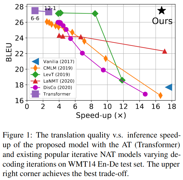
We can again see that most of the methods start at a similar speedup, but get much slower with the increasing translation quality. This is not the case of this paper that can preserve the quality of the AR model and the speedup of the fully NAR models.