This week I will review a paper that is not primarily about machine translation but about a neural architecture but can make a big impact on machine translation and natural language processing in general. This post is about Google’s Reformer, a neural architecture that is a more memory- and time-efficient version of the widely used Transformer architecture. In this post am trying to step-by-step explain what are the two main innovations that allow the model to time and save memory.

The Transformer is currently the most popular architecture for deep learning in natural language processing. It first became popular in machine translation in 2017. In 2018, it was used to train BERT, a pre-trained text representation that can be used in almost all NLP tasks and in 2019, many more cool Transformer-based models appeared.

Part of the Transformer’s strength probably comes from the fact that at each layer, it considers all possible combinations of all its inputs. The number of such combinations is quadratic in the sequence length, but it does not pose a time bottleneck thanks to intensive GPU parallelization. Still, you need enough memory to store the combinations. Also, the deeper the network is, the better performance you get, which also increases the memory requirements.

Reformer does two things differently from the standard Transformer

1. It adds a hashing function into the self-attention similarity computation, so only a small subset of states is actually used.

2. It uses a trick with so-called reversible layers, a brilliant idea using trivial algebra that causes that the model does not store values of activation function during training.

Self-Attention Locally Sensitive Hashing

The Transformer model is based on self-attention layers (this is the place where it considers all input combinations). In general, we can imagine the attention mechanism as probabilistic data retrieval. For a query, you want to retrieve some information about entries that you have in a data storage. Because we are in a neural network, both the queries and the data are vectors. We have some queries $Q = (q_1, \ldots, q_L)$, we compare them with some keys $K = (k_1, \ldots, k_L)$ and based on that comparison, we retrieve some values $V = (v_1, \ldots, v_L)$ that are associated with the keys.

In Transformers, each state corresponds to one input token (i.e., a word or a sub-word). Self-attention uses the same states as all queries, keys, and values. We can imagine the self-attention as collecting information that is encoded in some other hidden states (carried by other words). In each layer, each subword collects some (hopefully relevant) information from the other subwords and pass it further.

Because we might not want everything from other subwords, but only some particular information, we do so-called multi-head attention. In this setup, each head gets specialized for retrieving a specific kind of information. This “specialization” is achieved by linear projections of the states. The projection cannot add any information to the states, they only can suppress something or make something more prominent.

Now, we already projected our states and have three sets of states $Q$, $K$, and $V$. To make things computationally efficient, we treat the sets of vectors as matrices. The attention is computed as follows:

\[O = \text{softmax}\left( QK^\top / \sqrt{d} \right) V\]

$Q \in \mathbb{R}^{L \times d} = (q_1, \ldots, q_n)$ are $L$ query vectors, $K$ and $V$ are keys and values respectively. Here, the output of the softmax has size $L^2$ for a sequence of length $L$. This square is what the Reformer tries to get rid of.

Let us have a look at this from a perspective of a single query $q_i$ and re-write the dot-product (the $i$-th subword is looking for what subwords have).

\[o_i = \text{softmax} \left( \frac{q_i K}{\sqrt{d}}\right) V = \sum_{j=1 \ldots L} \left[ \text{softmax} \left( \frac{q_i K}{\sqrt{d}} \right) \right]_j \cdot v_j\]

If we further re-write the softmax, we get:

\[o_i = \sum_{j=1 \ldots L} \frac{\exp{q_i k_j / \sqrt{d}}} {\sum_{k=1 \ldots L}\exp{q_i k_k / \sqrt{d}}} v_j = \sum_{j=1 \ldots L} \exp \left( q_i k_j / \sqrt{d} - \log\sum_{k=1 \ldots L}\exp q_i k_k / \sqrt{d} \right )\]

In the paper, they call the log-sum-exp term the normalizer function $z$. If we further call the set of all indices $1 \ldots L$ as $\mathcal{P}(i)$, we get exactly the formulation that is in the paper, in Equation 2 on page 3.

\[o_i = \sum_{j \in \mathcal{P}_i} \exp \left( q_i k_j / \sqrt{d} - z(i, \mathcal{P}_i) \right)\] \[z(i, \mathcal{P}_i) = \log\sum_{j \in \mathcal{P}_i}\exp q_i k_j / \sqrt{d}\]

From analyses of learned Transformer models, we know that the attention distributions are usually quite sharp and only attend to few keys and the rest only gets a negligible probability. Now, if we were able to iterate over a substantially smaller set $\mathcal{P}(i)$ than $1 \ldots L$, we could save a lot of memory (and maybe some computation time as well). This is where the hashing comes into play.

The first part of the trick is to unify the projection of keys and queries. If we do this, for one head it holds that we are looking for few vectors that are the most similar to the query, vectors that belong to the same cluster (i.e., the set $\mathcal{P}(i)$ from the previous paragraph would be the cluster). Clustering is usually quite computationally demanding, but here it can be approximated by a fast hashing function. And in the best traditions of computer science, the clusters are called buckets.

For $b$ buckets, we sample $b/2$ random vectors and compare every query and key with those vectors using the dot product. There are two buckets for each random vector $r \in \mathbb{R}^d$: one for those which are the most similar to the vector $r$ and one for those which are the most similar to a negation of the vector. In the paper, they formally introduce a matrix $R \in \mathbb{R}^{d\times b/2} = \left( r_1, \ldots, r_{b/2} \right)$ and define the hashing function as:

\[h(x) = \arg\max\left([ xR; -xR ]\right) = \arg\max\left( xr_1, \ldots, xr_{b/2}, -xr_1, \ldots, -xr_{b/2} \right)\]

With such a hash function, we can do the attention only over the vectors that fall into the same bucket. In Equation 4 on page 4 of the paper, they formally write:

\[\mathcal{P}_i = \left\{ j: h(q_i) = h(k_j) \right\}\]

A hashing function like this might be useful if we computed everything vector by vector on CPU, but we need a fast GPU implementation. GPUs are good at matrix multiplications, dealing with sets of indices of different sizes does not sound like a task for GPU-accelerated computing. Here comes another trick for the rescue.

We sort the vectors according to their bucket number and split them into several equally large consecutive chunks. Vectors with the same hash number are likely to end up in the same chunk. The chunks should roughly correspond to the buckets because with random projections all buckets should be approximately the same size. Although, nothing is guaranteed, we can always have a bad luck with the random projection.

Within the chunks, we can do the self-attention as we always did but with much smaller matrices. To lower the chance that we miss something because of chunking, the attention also considers one chunk back as keys. In a language model where you only attend to previous positions anyway, this does not matter at all (given the sorting was stable). The chance that the state’s bucket-mate is two chunks away is very low. In a bidirectional encoder, it can play a more important role and a different strategy might be better.

In Figure 2 at the top of page 4, they illustrate the process like this:

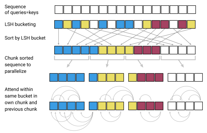
The sequence length in the illustration is 16. Without the hashing, we would need a similarity matrix of size 16 × 16 = 256 for each attention head at each layer. With the hashing, there are only 4 × 4 × 4 = 64 dot products. We got rid of the $L^2$-sized matrix, so now, the asymptotically most expensive part is sorting the states by the bucket numbers.

An important technical detail I did not mention and that is now obvious from the illustration is that we do not want to attend to vectors that ended up in the same chunk but got a different hash. Obviously, those need to be masked out. To be precise, we can rewrite the self-attention as the paper does in Equation 3 at the very bottom of page 3:

\[o_i = \sum_{j \in \mathcal{P}_i} \exp \left( q_i k_j / \sqrt{d} - m(j, \mathcal{P}_i) - z(i, \mathcal{P}_i) \right)\]

where $m(j, \mathcal{P}_i)$ is infinity if $j \not\in \mathcal{P}_i$ and 0 otherwise. In other words, if $i$ and $j$ are not in the same bucket, the probability we get from the softmax output will be zero at that position.

To further lower the chance that hashing will miss something, we can do the hashing multiple times (which can be done in parallel) and then just average what we get from the rounds.

Reversible layers

The other trick they use to improve memory efficiency is using reversible layers. But before I explain what exactly the reversible layers are, allow me to remind how back-propagation in neural networks works and how parameter gradients get computed.

Let us have a look at a simple example of logistic regression:

\[o = \sigma \left( \mathbf{W}\mathbf{x} + b \right)\]

The computation can be represented as a graph and computing the loss derivatives with respect to the parameters as a backward graph, a graph with reversed edges where the nodes represent derivatives of the operations in the original graph. $L$ is the loss function, let us say binary cross-entropy, and $y^\ast$ is the expected output of the network.

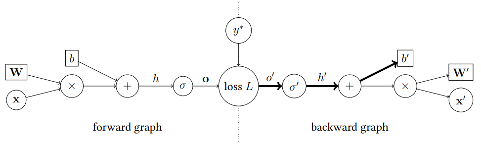
Looking at the graph, we can express the derivative of a loss function with respect to parameter $b$:

\[\frac{\partial L}{\partial b} = \frac{\partial L}{\partial o} \cdot \frac{\partial o}{\partial h} \cdot \frac{\partial h}{\partial b}\]

Now, let us have a look at the look at how terms look like:

\[\frac{\partial L}{\partial o} = \frac{o - y^\ast}{o(1-o)}\] \[\frac{\partial o}{\partial h} = \sigma(h)\left( 1 - \sigma(h) \right)\]

This example shows us that (almost) no matter what the function is, when doing the back-propagation, we need to remember what was the value of the node in the forward pass. And with Transformers, it means a lot of memory.

The standard Transformer uses residual connections. The purpose of residual connections is preventing the vanishing gradient problem. The trick is simple, we just sum the layer output with the layer input. When computing the loss derivative by back-propagation, there is always a path that only leads through the summation operations (plus maybe the few last other nodes), which are linear with respect to derivation. Other functions have derivatives that are often quite small or zero. Without the residual connections, you would (because of the chain rule) multiply the gradients by this small or zero derivatives so many times that it would eventually vanish. Such a path with summation operations is sometimes called the information highway.

The trick of the reversible layers is that if we have two information highways instead of one, so we can manage to compute the gradients without remembering the activation values. The architecture gets changed like this:

Expressed by formulas:

\[Y_1 = X_1 + \text{Attention}(X_2)\] \[Y_2 = X_2 + \text{FeedForward}(Y_1)\]

When doing the back-propagation, and computing gradients for the particular layer, we need the values of $X_1$ and $X_2$, but instead of remembering them, we can do:

\[X_2 = Y_2 - \text{FeedForward}(Y_1)\] \[X_1 = Y_1 - \text{Attention}(X_2)\]

Indeed, we need to call the $\text{FeedForward}$ and $\text{Attention}$ functions again which will cost us some time, but it will save a lot of memory. If we proceed to the layer before, the recently compute $X_1$ and $Y_2$ become $Y_1$ and $Y_2$ of that layer which can be again used to compute $X_2$ and $X_1$. We only need to remember the activations on the current layer and we can forget them as soon as we move in the back-propagation further.

At the beginning of the network, the input token embeddings are used as both $X_1$ and $X_2$. After the last layer, we just concatenate $Y_1$ and $Y_2$.

What will happen now

And this is it. This is how to save memory when training big Transformer models. The paper shows only a few experimental results (most importantly language modeling). They manage to show that with approximately the same model quality, it is much more memory-efficient and thanks to the hashing also faster than standard Transformers.

The Reformer was released together with an implementation in Google’s JAX. The paper was anonymously available on OpenReview since the end of September and even before publishing the non-anonymous pre-print on arXiv, there was a PyTorch re-implementation that gets seems to get better every day.

With Reformer, training of deeper NLP networks becomes more accessible. It will certainly allow more research on character-level processing and pre-trained representation outside big companies. Or maybe Google and Facebook will train even better and larger monster BERTs that still will be almost impossible for anyone else to develop and they will finally rule the world. We will see in 2020.